Models of Computation, Undecidability Complexity Classes

family of functions that should be regarded as “obviously computable,”

base functions

1. Composition
2. Primitive recursion
3. Minimization

Historically, the first two models of computation are

• the λ-calculus of Church (1935)
• the Turing machine (1936) of Turing.

the λ-calculus and Turing machines have the same “computing power,” and both compute exactly the class of computable functions in the sense of Herbrand–G¨odel–Kleene.

Partial Functions and RAM Programs

Partial Functions

Partial Functions:

• domain, dom(f)
• undefined

total function, iff dom(f)=A

RAM Program

A RAM program P (in linear form) consists of a finite sequence of instructions using a finite number of registers R1, . . . , Rp.

Instructions may optionally be labeled with line numbers
denoted as N1, . . . , Nq.
It is neither mandatory to label all instructions, nor to
use distinct line numbers!
Thus, the same line number can be used in more than
one line. As we will see later on, this makes it easier to
concatenate two di↵erent programs without performing a
renumbering of line numbers.
Every instruction has four fields, not necessarily all used.
The main field is the op-code.

Definition 1.2. RAM programs are constructed from seven types of instructions shown below

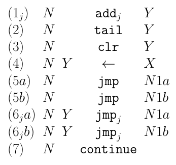
A RAM program P is a finite sequence of instructions as in Definition 1.2, and satisfying the following conditions:

• (1) For every jump instruction (conditional or not), the
  line number to be jumped to must exist in P.
• (2) The last instruction of a RAM program is a continue.

Definition 1.4. A RAM program P computes the partial function ': (⌃⇤)n ! ⌃⇤ if the following conditions hold: For every input (x1, . . . , xn) 2 (⌃⇤)n, having initialized the input registers R1, . . . , Rn with x1, . . . , xn, the program eventually halts i↵ '(x1, . . . , xn) is defined, and if and when P halts, the value of R1 is equal to '(x1, . . . , xn)

A partial function ' is RAM-computable i↵ it is computed by some RAM program.

For example, the following program computes the erase function E defined such that

RAM-computable

• One way of getting new programs from previous ones is via composition.
• Another one is by primitive recursion.

We will investigate these constructions after introducing another model of computation, Turing machines.

Remarkably, the classes of (partial) functions computed by RAM programs and by Turing machines are identical.

This is the class of partial computable functions, also called partial recursive functions, a term which is now considered old-fashion.

This class can be given several other definitions.

Lemma 1.1. Every RAM program can be converted to an equivalent program only using the following type of instructions:

Definition of a Turing Machine

A quintuple (p, a, b, m, q) 2 δ is called an instruction. It is also denoted as

p, a -> b, m, q

The effect of an instruction is to switch from state p to state q, overwrite the symbol currently scanned a with b, and move the read/write head either left or right, according to m.

Here is an example of a Turing machine.

Computations of Turing Machines

Instantaneous descriptions

The Primitive Recursive Functions

The base functions over ⌃ are the following functions:

For any partial or total function

Given any two partial or total functions g : Nm1 ! N and h: Nm+1 ! N (m 2), the partial or total function f : Nm ! N is defined by primitive recursion from g and h if f is given by

Primitive Recursive Predicates

An n-ary predicate P over N is any subset of Nn. We write that a tuple (x1,...,xn) satisfies P as (x1,...,xn) 2 P or as P(x1,...,xn). The characteristic function of a predicate P is the function CP : Nn ! {0, 1} defined by

A predicate P (over N) is primitive recursive i↵ its characteristic function CP is primitive recursive.