Interpolation

$R_1^0=[\hat i_1|\hat j_1|\hat k_1]$

Lengyel Chep 11.1-11.3

Single curve => global scheme

precises curve => local scheme

Explicit

Curves Representation

Three ways

Explicits

$y=f(x)$

Example: $y=\cos x$

properties

• generative
• Can only represent single-valued functions

Implicit

$f(x,y)=0$

Example: $x^2+y^2-z^2=0$

Properties

• Non-generative
• Can represent multi-valued functions

Parametric

$$x(t)=f(t)\\ y(t)=g(t)$$

where u is independent variable

Example:

$$x(t)=r\cos t\\ y(t)=r\sin t\\ t\in[0,2\pi]$$

Properties:

• generative
• Can represent multi-valued functions
• Different parametrization can produce the same path

Curves

Polynomial Curves

Monomial Form

$$f(u)=\vec a_0+\vec a_1u+\vec a_2u^2+...+\vec a_nu^n$$

where n=degree of polynomial curve (highest exponent)

• Linear
• Quadratic
• Cubic

$y=a_0+a_1u+a_2u^2+a_3u^3$=>monomial form

$\bar y=\bar a_0+\bar a_1 u+\bar a_2u^2+\bar a_3u^3$

Example

$$x(u)=1+6u-9u^2+4u^3\\ y(u)=-3u^2+4u^3\\ f(u)=\begin{pmatrix}x(u)\\y(u)\end{pmatrix} =\begin{pmatrix}1\\0\end{pmatrix}+ \begin{pmatrix}6\\0\end{pmatrix}u+ \begin{pmatrix}-9\\-3\end{pmatrix}u^2+ \begin{pmatrix}4\\4\end{pmatrix}u^3$$

Derivative

Continuity of Curves

• not continuous 不连续

• $c^0$自己连续，导数不连续

• $c^1$一阶导数连续，后面不连续

• $c^2$二阶导数连续，后面不连续

Note: Human visual system cannot distinguish discontinuities greater than to 2

Interpolation

General form (of curve and )

$$\begin{bmatrix} x(u)\\y(u)\\z(u) \end{bmatrix}=\vec{f}(u)=\sum_{i=0}^nb_iB_i^n(u)$$

$B_i^n(u)=$Basis functions of degree n (scalars not matrix)

Monomials: $B_i^n(u)\in\{1,u,u^2,...,u^n\}$

Linear Interpolation (n = 1)

$f(u)=b_0+b_1\cdot u$

Bézier curves

General form

$$\begin{pmatrix} x(u)\\y(u)\\z(u)\\... \end{pmatrix} =\vec{f}(u)=\sum_{i=0}^nb_iB_i^n(u)$$

n=1, linear

$\vec f(u)=\vec b_0(1-u)+\vec b_1(u)$

n=2, quadratic

$\vec f(u)=\vec b_0(1-u)^2+\vec b_12(1-u)+\vec b_2u^2$

n=3, cubic

$\vec f(u)=\vec b_0(1-u)^3+\vec b_13u(1-u)^2+\vec b_13u^2(1-u)+\vec b_3u^3$

General Form of Bernstein Polynomials of degree n

$$B_i^n(n)=C_i^n(1-u)^{n-i}u^i$$

control points

$\vec b_i$ control points

• b1, b2: slope

• b0, b3: point

让两个 curve 连接处平滑

几何意义：控制点就是这个曲线的 Convex Hull

Review, Lecture 7

Cubic Polynomials

monomials

$f(u)=c_0+c_1t+c_2t^2+c_3t^3$

Constructing Bezier Curves

De Casteljau Algorithm

Computes Bezier curve function $f(u)$ using successive linear interpolation

eg. want to know value of curve at u=0.25

$$\vec b_0^1=Lerp(\vec b_0,\vec b_1, u)\\ \vec b_1^1=Lerp(\vec b_1,\vec b_2, u)\\ \vec b_2^1=Lerp(\vec b_2,\vec b_3, u)\\ \vec b_0^2=Lerp(\vec b_0^1,\vec b_1^1, u)\\ \vec b_1^2=Lerp(\vec b_1^1,\vec b_2^1, u)\\ \vec b_0^3=Lerp(\vec b_0^2,\vec b_1^2, u)$$

where, $Lerp(a,b,u)=a(1-u)+bu, f(u)=\vec b_0^3$

Systolic(收缩) Array – associated with calculation of intermediate control points

Subdivision of Bezier Curve

$$B_{left}=\{\vec b_0,\vec b_0^1,\vec b_0^2,\vec b_0^3\}\\ B_{left}=\{\vec b_0^3,\vec b_1^2,\vec b_2^1,\vec b_2\}$$

Derivatives

$$\frac{df}{du}=f^1(u)=\sum_{i=0}^{n-1}n(\vec b_{i+1}-\vec b_i)B_i^{n-1}(u)$$

case n=3

$$f^1(u)=3(\vec b_1-\vec b_0)B_0^2(u)+3()...$$

Therefore,

$$\frac{df}{du}(0)=3(\vec b_1-\vec b_0)=\vec S_0\\ \frac{df}{du}(1)=3(\vec b_3-\vec b_2)=\vec S_1$$

Splines

Notations

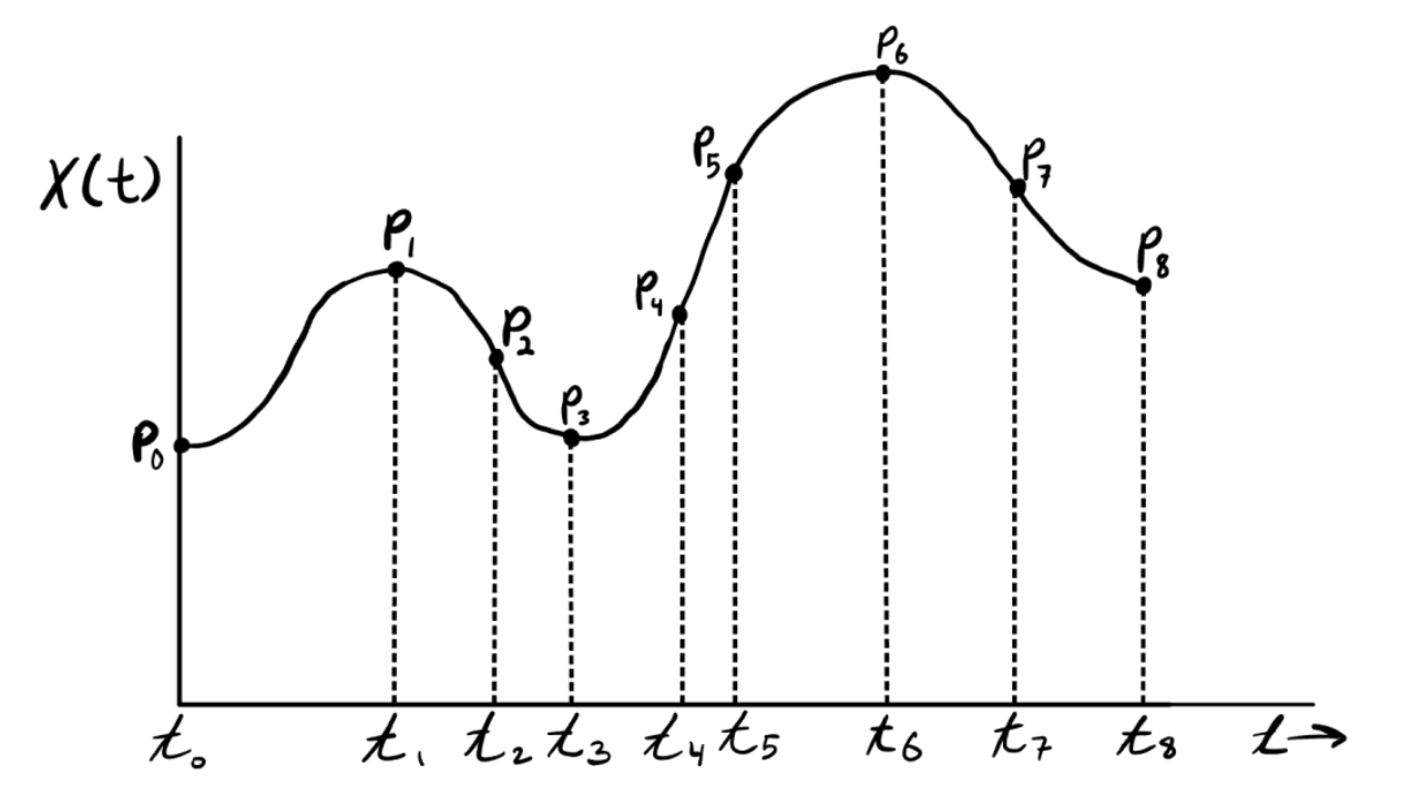
$t_i$: the knots of spline

$N$: # of curve segments

$n$: degree of the curve segments

$m=N+1=$number of points

Objective

Given

• a set of points $\{p_0,p_1,p_2,...,p_N\}$
• basis function polynomials of degree $\{B_0^n,B_1^n,\dots,B_n^n\}$ n

find the coefficient $b_i$ for the $j^{th}$ curve segment of the spline

$$f_j(t)=\begin{bmatrix} x(t)\\y(t)\\z(t) \end{bmatrix}=\sum_{i=0}^nb_iB_i^n(u)\\ where, u=\frac{t-t_j}{t_{j+1}-t_j}, j \in[0,N-1]$$

Catmull-Rom Splines

Centrol point: slope between two segment is same

C1 continuity

Use Bezier curves for each segment $j$

Cubic splines (n=3)

$$\vec f_j(t)=\vec b_0B^3_0(u)+\vec b_1B_1^3(u)+\vec b_2B_2^3(u)+\vec b_3B_3^3(u)$$

Control Point Array

Collect all the control points for spline into an array $C$

$$C=[\begin{array}{c:c}\vec b_0,\vec b_1,\vec b_2,\vec b_3&\vec b_0,\vec b_1,\vec b_2,\vec b_3&\vec b_0,\vec b_1,\vec b_2,\vec b_3]\end{array}\\ \vec f_j(t)=\sum_{j=0}^nC_{(n+1)j+i}B_j^n(u)$$

Computing control points for each curve segments (n=3, case)

$$\vec b_0=\vec P_j\\ \vec b_1=\vec b_0+\frac{1}{3}\vec S_0\\ \vec b_2=\vec b_3-\frac{1}{3}\vec S_1\\ \vec b_3=\vec P_{j+1}\\$$

Central difference

平均值 assume $\Delta t=1$

$$S_0=\frac{P_{i+1}-P_{i-1}}{2}\\ S_1=\frac{P_{i+2}-P_{i}}{2}$$

Endpoint

对于左右端点，特别的定义

• Left：$S_0=(\vec p_1-\vec p_0)$

• Right：$S_1=(\vec p_N-\vec p_{N-1})$

point value

to evaluate curve segment's particular point value in time t, need to compute B

1. Compute u, $u=\frac{t-t_j}{t_{j+1}-t_j}$
2. Use Bernstein polys to evaluate B
   • $B_0^3(u)=(1-u)^3$
   • $B_1^3(u)=3u(1-u)^2$

or

De Casteljau Algorithm

Monomial Formulation for cubic curves

m the Monomial form

$$\vec f(u)=\vec a_0+\vec a_1u+\vec a_2u^2+\vec a_3u^3=[]\\ \vec f(u)=G_{mon}M_{mon}U$$

Bezier Curve

$$\begin{align} f(u) &=\vec b_0+(3\vec b_1-3\vec b_0)u+(3\vec b_2-4\vec b_1+3\vec b_0)u^2+(\vec b_3-3\vec b_2+3\vec b_1-\vec b_0)u^3\\ &=[\vec b_0|\vec b_1|\vec b_2|\vec b_3] \begin{pmatrix} 1&-3&3&-1\\ 0&3&-6&3\\ 0&0&3&-3\\ 0&0&0&1 \end{pmatrix}\begin{pmatrix} 1\\ u\\ u^2\\ u^3 \end{pmatrix}\\ &=G_{Bez}M_{Bez}U \end{align}$$

What if I give the monomial coefficients () and value of

$$G_{Bez}=G_{Mon}M_{Mon}(M_{Bez})^{-1}$$

Hermite Curve

reworked Bezier curves

$$\vec h(u)=\vec p_0H_0^3(u)+\vec p_1H_3^3(u)+\vec p_0'H_1^3(u)+\vec p_1'H_2^3(u)$$

• $p_0$: left side of curve
• $p_1$: right side of curve
• $p_1'$: slope of left side of curve
• $p_2'$: slope of right side of curve

What is the basis functions H

Bezier curve derivatives

$$\vec f(u)=\\ \vec S_0=\frac{d\vec f(0)}{du}=3(\vec b_1-\vec b_0)$$

$$\vec h(u)=\vec f(u)=\begin{aligned} \vec b_0B_0^3+(b_0+\frac{1}{3}S_0)B_1^3+(b_3-\frac{1}{3}S_1)B_2^3+\vec b_3B_3^3 \end{aligned}$$

Hermite Spline

C2 continuity

General Case

$$\vec f_j(u)=\vec h_j(u)=\vec p_jH_0^3(u)+\vec p_{j+1}H_3^3(u)+\vec p_j'H_1^3(u)+\vec p_{j+1}'H_2^3(u)$$

1st Derivative:

$$\frac{d\vec f}{du}=f'=h'=\vec p_j(6u^2-6u)+\vec p_{j+1}(-6u^2+6u)+$$

2nd Derivative:

$$h''=$$

To have continuous 2nd derivative between segments

$$h_j''(1)=h_{j+1}''(0)$$

Constraint

$$p_j'+4p_{j+1}'+p_{j+2}'=3(p_{j+2}-p_j)$$

AC=D, C=A^{-1}D

Endpoint

Clamped Endpoint Conditions

S0, sn

natural spline

left and right side of curve 2nd derivative = 0

Spherical Interpolation (Slerp)

Interpolating Quaternion

$\|\vec p\|=1$

$\vec p=a\vec q_1+b\vec q_2$ linear combination of q1, q2

$\vec q_1\cdot\vec q_2=\cos\Omega$

$\vec q_1 \cdot\vec p=\cos\theta=\vec q_1 \cdot(a\vec q_1+b\vec q_2)=a+b\cos\Omega$

$\vec p\cdot\vec p=(a\vec q_1+b\vec q_2)\cdot(a\vec q_1+b\vec q_2)=a^2+2ab\cos\Omega+b^2=1$

=>

$$a=\frac{\sin(\Omega-\theta)}{\sin\Omega}\\ b=\frac{\sin\theta}{\sin\Omega}\\$$

let$\space \theta=u\Omega, u\in[0,1],\theta=\cos^{-1}(q_1\cdot q_2)$

$$\vec p=\frac{\sin((1-u)\Omega)}{\sin\Omega}\vec q_1+\frac{\sin(u\Omega)}{\sin\Omega}\vec q_2=Slerp(q_1,q_2,u)$$

Quaternion Splines

Cutmal-Rom

• slerp
• sdouble
• sbisect

use de Casteljau to evaluate spline at a given u

Statement

Assume want the equivalent of a Catmull-Rom spline

bezier

Geometric Interpretation of slope

Introduce 3

Operators

• $Double(a,b)=2*diff=a+2(b-a)$
• $Bisect(a,b)=\frac{(a+b)}{2}$
• $lerp(a,b,u)=(1-u)a+ub$

left slope

$$\vec p_{j+1}^d=Double(\vec p_{j-1},\vec p_j)\\ \vec p_{j+1}^b=Bisect(\vec p_{j+1},\vec p_{j+1}^d)$$

=>

$$\vec S_0=\vec p_{j+1}^b-\vec p_j=3(\vec b_1-\vec b_0)=3(\vec b_1-\vec p_j)\\ \vec b_1=\frac{1}{3}\vec p_{j+1}^b+\frac{2}{3}\vec p_j=lerp(p_j,p_{j+1}^b,\frac{1}{3})$$

right slope

$$\vec p_j^D=Double(\vec p_{j+2},\vec p_{j+1})\\ \vec p_j^B=Bisect(\vec p_j,\vec p_j^D)$$

=>

$$\vec S_1=p_{j+1}-p_j^B=3(b_3-b_2)=3(p_{j+1}-b_2)\\ b_2=xxx$$

Applied to circle

Operators

• $SBisect(a,b)=\frac{a+b}{\|a+b\|}$
• $SDouble(a,b)=2(a \cdot b)b-a$
• $Slerp(a,b,u)=$

---

Cubic Splines

$$\begin{aligned} \vec b_0&=\vec q_j\\ \vec b_1&=slerp(\vec q_{j},q_{j+1}^B,\frac{1}{3})\\ \vec b_2&=slerp(\vec q_{j+1},q_{j}^B,\frac{1}{3})\\ \vec b_3&=\vec q_{j+1} \end{aligned}$$

where

$$q_i^b=SBisect(q_i,q_i^d)\\ q_i^d=SDouble(q_{i+2},q_{i+1})\\ q_{i+1}^b=SBisect(q_{i+1}^d,q_{i+1})\\ q_{i+1}^d=SDouble(q_{i-1},q_{i})$$

edge case

Cubic Quaternion Catmul-Rom Splines

de Casteljau algorithm

$b_0^3=slerp(b_0^2,b_1^2,u)$

Shape Animation

2D Surfaces

surface

$(u,v)$

two tengant

normal: $\times$

Bilinear surface patch

2D linear interpolation

General form of Bilinear interpolation

$f(u,v)=\sum_{i=0}^1\sum_{j=0}^1B_i^1(u)B_j^1(v)b_{ij}$

2D Cubic Bezier

$f(u,v)=\sum_{i=0}^3\sum_{j=0}^3B_i^3(u)B_j^3(v)b_{ij}$

FFD (Free Form Deformation)

$(p-p_0)=f(u,v,w)=$

Jaccob matrix